Perbedaan Suka & Cinta

Anda tersenyum melihat orang yang anda suka, tapi mata anda akan berkaca-kaca melihat orang yang anda cinta.

Kata-katamu hanya keluar dari pikiran dengan orang yang kamu suka, tapi kata kata yang keluar berasal dari perasaan yang terdalam jika berhadapan dengan orang yang kamu cinta.

Jika orang yang kau cintai menangis, engkaupun akan ikut menangis disisinya. Jika orang yang kau sukai menangis, engkau hanya menghibur saja.

Perasaan cinta itu dimulai dari mata, sedangkan rasa suka dimulai dari telinga.
Jadi jika kau mau berhenti menyukai seseorang, cukup dengan menutup telinga.
Tapi apabila kau mencoba menutup matamu dari orang yang kau cintai, Cinta itu berubah menjadi tetesan air mata dan terus tinggal dihatimu.

Tetapi selain rasa suka dan rasa cinta…
Ada perasaan yang lebih mendalam.
Rasa yang tidak hilang .
Rasa yang tidak mudah berubah.
Rasa yang dapat membuatmu berkorban.
Rasa yang dapat membuatmu berkorban mau menderita untuknya..

Jika anda merasakan itu..
Selamat……
Berarti anda sedang menyayangi seseorang.
Dan berbahagialah kepada orang yang disayangi orang lain.

Theory of Anwar

One day an idea occurred to me when I was lecturing at the university of civil engineering about how to make compactions roads, we have what we call protector test, in which we sample and test soil used in fills in embankments. In this test we exclude and interpolate we have x and y. a hyperbole. We have a basic risk. We plot a curve and we put a line on the top of it. The line is the upper limit. Then I thought of the concept of “god limits” (hdud’illah). I returned here to the office and opened the Qur’an. Just as in mathematics we have five ways of representing limits. I found five cases in which the notion of God’s limit occurred. What they have in common is the idea that god has not set down the exact rules of conduct. But only the limits within which societies can create their own rules and laws, I have written about ideas of integrity (al-istiqama) and universal moral or ethical codes. The ideas was at first only a footnote in my last chapter, but I saw that it applied to my argument, so I corrected everything that in wrote about hudud’llah in the book in order to be consistent. Then I considered my argument to be sound.

Islamic legal theory came to recognize a variety of sources and methods from and through which the law might be derived. Those source from which the law may be derived are the Quran and sunna or example of the prophet. Both of which provide the subject matter of the law. Those sources through which the law may be derived represent either methods of legal reasoning and interpretation or the sanctioning instrument of consensus (ijma’), primacy of place within the hierarchy of all these sources is given to the Quran, followed by the sunna which. Though second in order of importance, provide the greatest bulk of material from which the law was derived. The third is consensus, a sanctioning instrument whereby the creative jurist, the mujtahids, representing the community at large, are considered to have reached an agreement, known retrospectively, on a technical legal ruling, thereby rendering it as conclusive and as epistemologically certain as any verse of the Quran and the sunna of the prophet . the certitude bestowed upon the case of law renders that case, together with its ruling, a material source on the basis of which a similar legal case may be solved. The mujtahids, authorized by devine revelation, are thus capable of transforming a ruling reached through human legal reasoning into the textual source by the very fact of their agreement on its validity. The processes of reasoning involved therein, subsumed under the rubric of qiyas, represent the fourth source of the law. Alternative methods of reasoning based on considerations of juristic preference (istihsan’) or public welfare and interest (istihlah) were of limited validity and were not infrequently the subject of controversy.

The two of modern reform we have identified, it is the religious utilitarianists who succeeded in having theire ideas implemented on the practical level,

Muhammad shahrur, whose recent work alkitab wal-quran advances some of the most controversial ideas in the middle east today, it is not difficult to see that his formal training as an engineer had great impact on his mode of analysis, in that in “re-reading” the quran and the suna he draws heavily on the natural sciences, particularly mathematics and physics. His, then is unique contribution to the reinterpretation of the quran and the sunna in particular, and to law as a comprehensive system in general. Although shahrur modestly claims that his work represents no more than a “contemporary reading” of the quran, being in no way an exegetical or a legal work. It is impressive in that it offers both depth and range, virtually unparalleled in modern writings on the subject

Shahrur maintains that the quran having been constantly “preserved” by divine power, is as much the property of later generations as that of earlier or even the earliest generations, since each generation bestows on the quran an interpretation emanating from the particular reality in which it lives, we in the twentieth century, are entitled to confer on the “remembrance” an interpretation that reflects the condition of this age. In this sense, modern muslim are more qualified to understand the quran for their own purposes and exigencies than earlier generations were. Thus, traditional interpretation of the quran must not be taken as binding upon modern muslim societies. But shahrur goes further: modern muslims are better equipped to understand the meaning of revelation than their classical and medieval counterparts because they are far more “cultured”. The quran speaks of the Bedouins as having been “ more hard is disbelief and hypocrisy “ than the other arabs who possessed higher culture and civilization, and “likely to be ignorant of the limit which god revealed to his messenger “ (9:97) . the Quranic criterion of a proper comprehension of the revealed text is thus a level of high culture which the Bedouins were thought to have lacked. Since muslims in the twentieth century enjoy a higher level of culture and scientific knowledge than their predecessors, then they are better equipped to understand revelation than these predecessors were.

Having arrogated to his generation the superior right to interpret the remembrance, shahrur goes on the draw a crucial distinction between what he calls the quran and the book (these two words constituting the title of his work). This distinction directly emanates from yet another distinction, namely between the function of Muhammad received a body of information having to do with prophecy, religion and the like, as messenger and as prophet. As prophet Muhammad received a body of information having to do with prophecy, religion and the like. As messenger, he was the recipient of a corpus of legal instructions, in addition to that information he received as a prophet. The function of the prophet, then is religious, whereas that of the messenger is legal. Now prophetic information is textually ambiguous, capable of varying interpretation. This is the quran. On the other hand, the legal subject matter is univocal, but nevertheless capable of being subjected to ijtihad. This is the book.

In order to understand the legal message, it is necessary to draw another fundamental distinction between two contradictory, yet complementary attributes found in the book, these are straightness (istiqama) and curvature (hanifiyya). It is to be noted here that our English rendering of these two Arabic terms does not represent their immediate meaning as they have been traditionally understood but rather as shahrur perceives them by means of his own linguistics derivation. Listing numerous quranic verses in which these two terms occur, he concludes that the meaning of hanifiyya is derivation from straight path or from a linearity. The opposite of hanifiyya is istiqoma, the letter being the quality of being straight or of following a linear path.

Both of these attributes are integral to the message, coexisting in a symbiotic relationship. Curvature is a natural quality, meaning that it is intrinsic to human nature as it exist in the material, objective world. Physical laws show that things do not occur in a linear, but rather in a non – linear, fashion. Motion in the natural world, for instance, is characterized by curves. All thing, from minute electrons to the colossal galaxies, move in curves. In line with this perception of nature, curvature in law is seen as representing the quality of non linear movement, where customs, habits and social traditions tend to exist in harmony with the needs of particular societies, needs that tend to change from one society to another and, diachronically, within a society. It is for the purpose of controlling and restraining this change that “ straightness” becomes indispensable for maintaining a legal order, but unlike curvature, straightness is not natural quality. Rather it is divinely ordained in order for it to coexist with curvature and to partake in the ordering of human societies. Thus curvature stand in need of straightness, as attested in 1:5 where man is represented as seeking the guidance of god by imploring him to “show us the straight path” on the other hand, there exists no quranic verse, shahrur maintains, in which man is portrayed as seeking curvature (hanifiyya) because curvature is pre-existing in the natural order.

The relationship between curvature and straightness is thus wholly dialectical, where constants and permutations are intertwined. This dialectic is significant because it indicates that the law is adaptable to all times and places (salih li-kulli zaman wa-makan). But what is the form of straightness that god revealed in order to complement cvurvature? Here shahrur advances the crux of his theory, which we may call the theory of limits (hudud). Ultimately, then man moves in curvature within these limits which represent straightness.

The theory of limits may be describes as follows ; it is the divine decree, expressed in the book and the sunna, which sets a lower and an upper limit for all human actions; the lower limit represents the minimum required by the law in a particular case, and the upper limit the maximum. Just as nothing short of the minimum is legally admissible, so nothing above the maximum may be deemed lawful. Once these limits are transcended, penalties become warrantable, in proportion to the violation committed.

Shahrur distinguishes six types of limits, the first of which is the lower

coba

shahrour maintains that the qur'an having been constantly "preserved" by divine power

Quadratic equation

From Wikipedia, the free encyclopedia
Jump to: navigation, search
This article is about quadratic equations and their solutions. For more general information about quadratic functions, see Quadratic function.

In mathematics, a quadratic equation is a polynomial equation of the second degree. The general form is

ax^2+bx+c=0,\,\!


where a ≠ 0. (If a = 0, the equation becomes a linear equation.)

The letters a, b, and c are called coefficients: the quadratic coefficient a is the coefficient of x2, the linear coefficient b is the coefficient of x, and c is the constant coefficient, also called the free term or constant term.

Quadratic equations are called quadratic because quadratus is Latin for "square"; in the leading term the variable is squared.
Plots of real-valued quadratic function ax2 + bx + c, varying each coefficient separately
Contents
[hide]

* 1 Quadratic formula
* 2 Discriminant
* 3 Geometry
* 4 Examples
* 5 Quadratic factorization
* 6 Application to higher-degree equations
* 7 History
* 8 Derivation
* 9 Alternative formula
* 10 Floating point implementation
* 11 Viète's formulas
* 12 Generalizations
o 12.1 Characteristic 2
* 13 See also
* 14 Notes
* 15 References
* 16 External links

[edit] Quadratic formula

A quadratic equation with real or complex coefficients has two, but not necessarily distinct, solutions, called roots, which may or may not be real, given by the quadratic formula:

x = \frac{-b \pm \sqrt {b^2-4ac}}{2a} ,

where the symbol "±" indicates that both

x_+ = \frac{-b + \sqrt {b^2-4ac}}{2a} and \ x_- = \frac{-b - \sqrt {b^2-4ac}}{2a}

are solutions.

[edit] Discriminant
Example discriminant signs
■ <0:>0: 3⁄2x2+1⁄2x−4⁄3

In the above formula, the expression underneath the square root sign:

\Delta = b^2 - 4ac , \,\!

is called the discriminant of the quadratic equation.

A quadratic equation with real coefficients can have either one or two distinct real roots, or two distinct complex roots. In this case the discriminant determines the number and nature of the roots. There are three cases:

* If the discriminant is positive, there are two distinct roots, both of which are real numbers. For quadratic equations with integer coefficients, if the discriminant is a perfect square, then the roots are rational numbers—in other cases they may be quadratic irrationals.
* If the discriminant is zero, there is exactly one distinct root, and that root is a real number. Sometimes called a double root, its value is:

x = -\frac{b}{2a} . \,\!

* If the discriminant is negative, there are no real roots. Rather, there are two distinct (non-real) complex roots, which are complex conjugates of each other:

\begin{align} x &= \frac{-b}{2a} + i \frac{\sqrt {4ac - b^2}}{2a} , \\ x &= \frac{-b}{2a} - i \frac{\sqrt {4ac - b^2}}{2a}. \end{align}

Thus the roots are distinct if and only if the discriminant is non-zero, and the roots are real if and only if the discriminant is non-negative.

[edit] Geometry
For the quadratic function:
f (x) = x2 − x − 2 = (x + 1)(x − 2) of a real variable x, the x-coordinates of the points where the graph intersects the x-axis, x = −1 and x = 2, are the roots of the quadratic equation: x2 − x − 2 = 0.

The roots of the quadratic equation

ax^2+bx+c=0,\,

are also the zeros of the quadratic function:

f(x) = ax^2+bx+c,\,

since they are the values of x for which

f(x) = 0.\,

If a, b, and c are real numbers and the domain of f is the set of real numbers, then the zeros of f are exactly the x-coordinates of the points where the graph touches the x-axis.

It follows from the above that, if the discriminant is positive, the graph touches the x-axis at two points, if zero, the graph touches at one point, and if negative, the graph does not touch the x-axis.

[edit] Examples

* 7x + 15 − 2x2 = 0 has a strictly positive discriminant Δ = 169 and therefore has two real solutions:

x_1=\frac{-7-\sqrt{169}}{2\cdot(-2)}=\frac{-7-13}{-4} =\frac{20}{4}= 5

and

x_2=\frac{-7+\sqrt{169}}{2\cdot(-2)} = \frac{-7+13}{-4}=\frac{6}{-4}=-\frac{3}{2}.

* x2 − 2x + 1 = 0 has a discriminant Δ whose value is zero, therefore it has a double solutionx_0=-\tfrac{-2}{2}=1
* x2 + 3x + 3 = 0 has no real solution because Δ = − 3 < 0. But it has two complex solutions x_1\! and x_2\!:

x_1 = \frac{-3 - \sqrt{3} i}{2}\text{ and }x_2 = \frac{-3 + \sqrt{3} i}{2}.

[edit] Quadratic factorization

The term

x - r\,

is a factor of the polynomial

ax^2+bx+c, \

if and only if r is a root of the quadratic equation

ax^2+bx+c=0. \

It follows from the quadratic formula that

ax^2+bx+c = a \left( x - \frac{-b + \sqrt {b^2-4ac}}{2a} \right) \left( x - \frac{-b - \sqrt {b^2-4ac}}{2a} \right).

In the special case where the quadratic has only one distinct root (i.e. the discriminant is zero), the quadratic polynomial can be factored as

ax^2+bx+c = a \left( x + \frac{b}{2a} \right)^2.\,\!

[edit] Application to higher-degree equations

Certain higher-degree equations can be brought into quadratic form and solved that way. For example, the 6th-degree equation in x:

x^6 - 4x^3 + 8 = 0\,

can be rewritten as:

(x^3)^2 - 4(x^3) + 8 = 0\,,

or, equivalently, as a quadratic equation in a new variable u:

u^2 - 4u + 8 = 0,\,

where

u = x^3.\,

Solving the quadratic equation for u results in the two solutions:

u = 2 \pm 2i.

Thus

x^3 = 2 \pm 2i\,.

Concentrating on finding the three cube roots of 2 + 2i – the other three solutions for x will be their complex conjugates – rewriting the right-hand side using Euler's formula:

x^3 = 2^{\tfrac{3}{2}}e^{\tfrac{1}{4}\pi i} = 2^{\tfrac{3}{2}}e^{\tfrac{8k+1}{4}\pi i}\,

(since e2kπi = 1), gives the three solutions:

x = 2^{\tfrac{1}{2}}e^{\tfrac{8k+1}{12}\pi i}\,,~k = 0, 1, 2\,.

Using Eulers' formula again together with trigonometric identities such as cos(π/12) = (√2 + √6) / 4, and adding the complex conjugates, gives the complete collection of solutions as:

x_{1,2} = -1 \pm i,\,
x_{3,4} = \frac{1 + \sqrt{3}}{2} \pm \frac{1 - \sqrt{3}}{2}i\,

and

x_{5,6} = \frac{1 - \sqrt{3}}{2} \pm \frac{1 + \sqrt{3}}{2}i.\,

[edit] History

The Babylonians, as early as 1800 BC (displayed on Old Babylonian clay tablets) could solve a pair of simultaneous equations of the form:

x+y=p,\ \ xy=q \

which are equivalent to the equation:[1]

\ x^2+q=px

The original pair of equations were solved as follows:

1. Form \frac{x+y}{2}
2. Form \left(\frac{x+y}{2}\right)^2
3. Form \left(\frac{x+y}{2}\right)^2 - xy
4. Form \sqrt{\left(\frac{x+y}{2}\right)^2 - xy} = \frac{x-y}{2}
5. Find x,\ y by inspection of the values in (1) and (4).[2]

In the Sulba Sutras in ancient India circa 8th century BCE quadratic equations of the form ax2 = c and ax2 + bx = c were explored using geometric methods. Babylonian mathematicians from circa 400 BCE and Chinese mathematicians from circa 200 BCE used the method of completing the square to solve quadratic equations with positive roots, but did not have a general formula. Euclid, the Greek mathematician, produced a more abstract geometrical method around 300 BCE.

In 628 CE, Brahmagupta, an Indian mathematician, gave the first explicit (although still not completely general) solution of the quadratic equation:

\ ax^2+bx=c

“ To the absolute number multiplied by four times the [coefficient of the] square, add the square of the [coefficient of the] middle term; the square root of the same, less the [coefficient of the] middle term, being divided by twice the [coefficient of the] square is the value. (Brahmasphutasiddhanta (Colebrook translation, 1817, page 346)[3] ”

This is equivalent to:

x = \frac{\sqrt{4ac+b^2}-b}{2a}.

The Bakhshali Manuscript dated to have been written in India in the 7th century CE contained an algebraic formula for solving quadratic equations, as well as quadratic indeterminate equations (originally of type ax/c = y). Mohammad bin Musa Al-kwarismi (Persia, 9th century) developed a set of formulae that worked for positive solutions. His work was based on Brahmagupta. A Catalan Jewish mathematician Abraham bar Hiyya Ha-Nasi (also known by the Latin name Savasorda) introduced the complete solution to Europe in his book Liber embadorum in the 12th century. Bhāskara II (1114–1185), an Indian mathematician–astronomer, gave the first general solution to the quadratic equation with two roots.[4]

The writing of the Chinese mathematician Yang Hui (1238-1298 AD) represents the first in which quadratic equations with negative coefficients of 'x' appear, although he attributes this to the earlier Liu Yi. The first appearance of the general solution in the modern mathematical literature is evidently in an 1896 paper by Henry Heaton[5].

[edit] Derivation

The quadratic formula can be derived by the method of completing the square, so as to make use of the algebraic identity:

x^2+2xh+h^2 = (x+h)^2.\,\!

Dividing the quadratic equation

ax^2+bx+c=0 \,\!

by a (which is allowed because a is non-zero), gives:

x^2 + \frac{b}{a} x + \frac{c}{a}=0,\,\!

or

x^2 + \frac{b}{a} x= -\frac{c}{a} \qquad (1)

The quadratic equation is now in a form to which the method of completing the square can be applied. To "complete the square" is to find some constant k such that

x^2 + \frac{b}{a}x + k = x^2+2xh+h^2,\,\!

for another constant h. In order for these equations to be true,

\frac{b}{a} = 2h\!

or

h = \frac{b}{2a}\,\!

and

k = h^2,\,\!

thus

k = \frac{b^2}{4a^2}.\,\!

Adding this constant to equation (1) produces

x^2+\frac{b}{a}x+\frac{b^2}{4a^2}=-\frac{c}{a}+\frac{b^2}{4a^2}.\,\!

The left side is now a perfect square because

x^2+\frac{b}{a}x+\frac{b^2}{4a^2} = \left( x + \frac{b}{2a} \right)^2

The right side can be written as a single fraction, with common denominator 4a2. This gives

\left(x+\frac{b}{2a}\right)^2=\frac{b^2-4ac}{4a^2}.

Taking the square root of both sides yields

\left|x+\frac{b}{2a}\right| = \frac{\sqrt{b^2-4ac\ }}{|2a|}\Rightarrow x+\frac{b}{2a}=\pm\frac{\sqrt{b^2-4ac\ }}{2a}.

Isolating x, gives

x=-\frac{b}{2a}\pm\frac{\sqrt{b^2-4ac\ }}{2a}=\frac{-b\pm\sqrt{b^2-4ac\ }}{2a}.

[edit] Alternative formula

In some situations it is preferable to express the roots in an alternate form.

x =\frac{2c}{-b \mp \sqrt {b^2-4ac\ }} .

This alternative requires c to be nonzero; for, if c is zero, the formula correctly gives zero as one root, but fails to give any second, non-zero root. Instead, one of the two choices for ∓ produces a division by zero, which is undefined.

The roots are the same regardless of which expression we use; the alternate form is merely an algebraic variation of the common form:

\begin{align} \frac{-b + \sqrt {b^2-4ac\ }}{2a} &{}= \frac{-b + \sqrt {b^2-4ac\ }}{2a} \cdot \frac{-b - \sqrt {b^2-4ac\ }}{-b - \sqrt {b^2-4ac\ }} \\ &{}= \frac{4ac}{2a \left ( -b - \sqrt {b^2-4ac} \right ) } \\ &{}=\frac{2c}{-b - \sqrt {b^2-4ac\ }}. \end{align}

The alternative formula can reduce loss of precision in the numerical evaluation of the roots, which may be a problem if one of the roots is much smaller than the other in absolute magnitude. The problem of c possibly being zero can be avoided by using a mixed approach:

x_1 = \frac{-b - \sgn b \,\sqrt {b^2-4ac}}{2a},
x_2 = \frac{c}{ax_1}.

Here sgn denotes the sign function.

[edit] Floating point implementation

A careful floating point computer implementation differs a little from both forms to produce a robust result. Assuming the discriminant, b2 − 4ac, is positive and b is nonzero, the code will be something like the following.

t := -\tfrac12 \big( b + \sgn(b) \sqrt{b^2-4ac} \big) \,\!
r_1 := t/a \,\!
r_2 := c/t \,\!

Here sgn(b) is the sign function, where sgn(b) is 1 if b is positive and −1 if b is negative; its use ensures that the quantities added are of the same sign, avoiding catastrophic cancellation. The computation of r2 uses the fact that the product of the roots is c/a.

See Numerical Recipes in C, Section 5.6: "Quadratic and Cubic Equations".

[edit] Viète's formulas

Viète's formulas give a simple relation between the roots of a polynomial and its coefficients. In the case of the quadratic polynomial, they take the following form:

x_+ + x_- = -\frac{b}{a}

and

x_+ \cdot x_- = \frac{c}{a}.

The first formula above yields a convenient expression when graphing a quadratic function. Since the graph is symmetric with respect to a vertical line through the vertex, when there are two real roots the vertex’s x-coordinate is located at the average of the roots (or intercepts). Thus the x-coordinate of the vertex is given by the expression:

x_V = \frac {x_+ + x_-} {2} = -\frac{b}{2a}.

The y-coordinate can be obtained by substituting the above result into the given quadratic equation, giving

y_V = - \frac{b^2}{4a} + c = - \frac{ b^2 - 4ac} {4a}.

[edit] Generalizations

The formula and its derivation remain correct if the coefficients a, b and c are complex numbers, or more generally members of any field whose characteristic is not 2. (In a field of characteristic 2, the element 2a is zero and it is impossible to divide by it.)

The symbol

\pm \sqrt {b^2-4ac}

in the formula should be understood as "either of the two elements whose square is

b^2-4ac,\,

if such elements exist. In some fields, some elements have no square roots and some have two; only zero has just one square root, except in fields of characteristic 2. Note that even if a field does not contain a square root of some number, there is always a quadratic extension field which does, so the quadratic formula will always make sense as a formula in that extension field.

[edit] Characteristic 2

In a field of characteristic 2, the quadratic formula, which relies on 2 being a unit, does not hold. Consider the monic quadratic polynomial

\displaystyle x^{2} + bx + c

over a field of characteristic 2. If b = 0, then the solution reduces to extracting a square root, so the solution is

\displaystyle x = \sqrt{c}

and note that there is only one root since

\displaystyle -\sqrt{c} = -\sqrt{c} + 2\sqrt{c} = \sqrt{c}.

In summary,

\displaystyle x^{2} + c = (x + \sqrt{c})^{2}.

See quadratic residue for more information about extracting square roots in finite fields.

In the case that b ≠ 0, there are two distinct roots, but if the polynomial is irreducible, they cannot be expressed in terms of square roots of numbers in the coefficient field. Instead, define the 2-root R(c) of c to be a root of the polynomial x2 + x + c, an element of the splitting field of that polynomial. One verifies that R(c) + 1 is also a root. In terms of the 2-root operation, the two roots of the (non-monic) quadratic ax2 + bx + c are

\frac{b}{a}R\left(\frac{ac}{b^2}\right)

and

\frac{b}{a}\left(R\left(\frac{ac}{b^2}\right)+1\right).

For example, let a denote a multiplicative generator of the group of units of F4, the Galois field of order four (thus a and a + 1 are roots of x2 + x + 1 over F4). Because (a + 1)2 = a, a + 1 is the unique solution of the quadratic equation x2 + a = 0. On the other hand, the polynomial x + ax + 1 is irreducible over F4, but splits over F16, where it has the two roots ab and ab + a, where b is a root of x2 + x + a in F16.

This is a special case of Artin-Schreier theory.

Fungsi

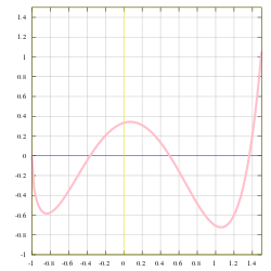
Graph of example function,

The mathematical concept of a function expresses dependence between two quantities, one of which is known (the independent variable, argument of the function, or its "input") and the other produced (the dependent variable, value of the function, or "output"). A function associates a single output to each input element drawn from a fixed set, such as the real numbers (), although different inputs may have the same output.

There are many ways to give a function: by a formula, by a plot or graph, by an algorithm that computes it, or by a description of its properties. Sometimes, a function is described through its relationship to other functions (see, for example, inverse function). In applied disciplines, functions are frequently specified by their tables of values or by a formula. Not all types of description can be given for every possible function, and one must make a firm distinction between the function itself and multiple ways of presenting or visualizing it.

One idea of enormous importance in all of mathematics is composition of functions: if z is a function of y and y is a function of x, then z is a function of x. We may describe it informally by saying that the composite function is obtained by using the output of the first function as the input of the second one. This feature of functions distinguishes them from other mathematical constructs, such as numbers or figures, and provides the theory of functions with its most powerful structure.

Contents [hide] 1 Introduction 2 Definitions 2.1 Intuitive definitions 2.2 Set-theoretical definitions 3 History 4 Vocabulary 4.1 Restrictions and extensions 5 Notation 6 Function composition 7 Identity function 8 Inverse function 9 Specifying a function 9.1 Computability 9.2 Functions with multiple inputs and outputs 9.2.1 Binary operations 10 Function spaces 11 Pointwise operations 12 Other properties 13 See also 14 References 14.1 Notes 14.2 Sources 15 External links

[edit] Introduction

Functions play a fundamental role in all areas of mathematics, as well as in other sciences and engineering. However, the intuition pertaining to functions, notation, and even the very meaning of the term "function" varies between the fields. More abstract areas of mathematics, such as set theory, consider very general types of functions, which may not be specified by a concrete rule and are not governed by any familiar principles. The characteristic property of a function in the most abstract sense is that it relates exactly one output to each of its admissible inputs. Such functions need not involve numbers and may, for example, associate each of a set of words with its own first letter.

Functions in algebra are usually expressed in terms of algebraic operations. Functions studied in analysis, such as the exponential function, may have additional properties arising from continuity of space, but in the most general case cannot be defined by a single formula. Analytic functions in complex analysis may be defined fairly concretely through their series expansions. On the other hand, in lambda calculus, function is a primitive concept, instead of being defined in terms of set theory. The terms transformation and mapping are often synonymous with function. In some contexts, however, they differ slightly. In the first case, the term transformation usually applies to functions whose inputs and outputs are elements of the same set or more general structure. Thus, we speak of linear transformations from a vector space into itself and of symmetry transformations of a geometric object or a pattern. In the second case, used to describe sets whose nature is arbitrary, the term mapping is the most general concept of function.

In traditional calculus, a function is defined as a relation between two terms called variables because their values vary. Call the terms, for example, x and y. If every value of x is associated with exactly one value of y, then y is said to be a function of x. It is customary to use x for what is called the "independent variable," and y for what is called the "dependent variable" because its value depends on the value of x.^[1]

Restated, mathematical functions are denoted frequently by letters, and the standard notation for the output of a function ƒ with the input x is ƒ(x). A function may be defined only for certain inputs, and the collection of all acceptable inputs of the function is called its domain. The set of all resulting outputs is called the range of the function. However, in many fields, it is also important to specify the codomain of a function, which contains the range, but need not be equal to it. The distinction between range and codomain lets us ask whether the two happen to be equal, which in particular cases may be a question of some mathematical interest.

For example, the expression ƒ(x) = x² describes a function ƒ of a variable x, which, depending on the context, may be an integer, a real or complex number or even an element of a group. Let us specify that x is an integer; then this function relates each input, x, with a single output, x², obtained from x by squaring. Thus, the input of 3 is related to the output of 9, the input of 1 to the output of 1, and the input of −2 to the output of 4, and we write ƒ(3) = 9, ƒ(1)=1, ƒ(−2)=4. Since every integer can be squared, the domain of this function consists of all integers, while its range is the set of perfect squares. If we choose integers as the codomain as well, we find that many numbers, such as 2, 3, and 6, are in the codomain but not the range.

It is a usual practice in mathematics to introduce functions with temporary names like ƒ; in the next paragraph we might define ƒ(x) = 2x+1, and then ƒ(3) = 7. When a name for the function is not needed, often the form y = x² is used.

If we use a function often, we may give it a more permanent name as, for example,

The essential property of a function is that for each input there must be a unique output. Thus, for example, the formula

does not define a real function of a positive real variable, because it assigns two outputs to each number: the square roots of 9 are 3 and −3. To make the square root a real function, we must specify, which square root to choose. The definition

for any positive input chooses the positive square root as an output.

As mentioned above, a function need not involve numbers. By way of examples, consider the function that associates with each word its first letter or the function that associates with each triangle its area.

[edit] Definitions

Because functions are used in so many areas of mathematics, and in so many different ways, no single definition of function has been universally adopted. Some definitions are elementary, while others use technical language that may obscure the intuitive notion. Formal definitions are set theoretical and, though there are variations, rely on the concept of relation. Intuitively, a function is a way to assign to each element of a given set (the domain or source) exactly one element of another given set (the codomain or target).

[edit] Intuitive definitions

One simple intuitive definition, for functions on numbers, says:

• A function is given by an arithmetic expression describing how one number depends on another.

An example of such a function is y = 5x−20x³+16x⁵, where the value of y depends on the value of x. This is entirely satisfactory for parts of elementary mathematics, but is too clumsy and restrictive for more advanced areas. For example, the cosine function used in trigonometry cannot be written in this way; the best we can do is an infinite series,

That said, if we are willing to accept series as an extended sense of "arithmetic expression", we have a definition that served mathematics reasonably well for hundreds of years.

Eventually the gradual transformation of intuitive "calculus" into formal "analysis" brought the need for a broader definition. The emphasis shifted from how a function was presented — as a formula or rule — to a more abstract concept. Part of the new foundation was the use of sets, so that functions were no longer restricted to numbers. Thus we can say that

• A function ƒ from a set X to a set Y associates to each element x in X an element y = ƒ(x) in Y.

Note that X and Y need not be different sets; it is possible to have a function from a set to itself. Although it is possible to interpret the term "associates" in this definition with a concrete rule for the association, it is essential to move beyond that restriction. For example, we can sometimes prove that a function with certain properties exists, yet not be able to give any explicit rule for the association. In fact, in some cases it is impossible to give an explicit rule producing a specific y for each x, even though such a function exists. In the context of functions defined on arbitrary sets, it is not even clear how the phrase "explicit rule" should be interpreted.

[edit] Set-theoretical definitions

As functions take on new roles and find new uses, the relationship of the function to the sets requires more precision. Perhaps every element in Y is associated with some x, perhaps not. In some parts of mathematics, including recursion theory and functional analysis, it is convenient to allow values of x with no association (in this case, the term partial function is often used). To be able to discuss such distinctions, many authors split a function into three parts, each a set:

• A function ƒ is an ordered triple of sets (F,X,Y) with restrictions, where

  F (the graph) is a set of ordered pairs (x,y),

  X (the source) contains all the first elements of F and perhaps more, and

  Y (the target) contains all the second elements of F and perhaps more.

The most common restrictions are that F pairs each x with just one y, and that X is just the set of first elements of F and no more. The terminology total function is sometimes used to indicate that every element of X does appear as the first element of an ordered pair in F; see partial function. In most contexts in mathematics, "function" is used as a synonym for "total function".

When no restrictions are placed on F, we speak of a relation between X and Y rather than a function. The relation is "single-valued" when the first restriction holds: (x,y₁)∈F and (x,y₂)∈F together imply y₁ = y₂. Relations that are not single valued are sometimes called multivalued functions. A relation is "total" when a second restriction holds: if x∈X then (x,y)∈F for some y. Thus we can also say that

• A function from X to Y is a single-valued, total relation between X and Y.^[2]

The range of F, and of ƒ, is the set of all second elements of F; it is often denoted by rng ƒ. The domain of F is the set of all first elements of F; it is often denoted by dom ƒ. There are two common definitions for the domain of ƒ some authors define it as the domain of F, while others define it as the source of F.

The target Y of ƒ is also called the codomain of ƒ, denoted by cod ƒ; and the range of ƒ is also called the image of ƒ, denoted by im ƒ. The notation ƒ:X→Y indicates that ƒ is a function with domain X and codomain Y.

Some authors omit the source and target as unnecessary data. Indeed, given only the graph F, one can construct a suitable triple by taking dom F to be the source and rng F to be the target; this automatically causes F to be total. However, most authors in advanced mathematics prefer the greater power of expression afforded by the triple, especially the distinction it allows between range and codomain.

Incidentally, the ordered pairs and triples we have used are not distinct from sets; we can easily represent them within set theory. For example, we can use {{x},{x,y}} for the pair (x,y). Then for a triple (x,y,z) we can use the pair ((x,y),z). An important construction is the Cartesian product of sets X and Y, denoted by X×Y, which is the set of all possible ordered pairs (x,y) with x∈X and y∈Y. We can also construct the set of all possible functions from set X to set Y, which we denote by either [X→Y] or Y^X.

We now have tremendous flexibility. By using pairs for X we can treat, say, subtraction of integers as a function, sub:Z×Z→Z. By using pairs for Y we can draw a planar curve using a function, crv:R→R×R. On the unit interval, I, we can have a function defined to be one at rational numbers and zero otherwise, rat:I→2. By using functions for X we can consider a definite integral over the unit interval to be a function, int:[I→R]→R.

Yet we still are not satisfied. We may want even more generality in some cases, like a function whose integral is a step function; thus we define so-called generalized functions. We may want less generality, like a function we can always actually use to get a definite answer; thus we define primitive recursive functions and then limit ourselves to those we can prove are effectively computable. Or we may want to relate not just sets, but algebraic structures, complete with operations; thus we define homomorphisms.

[edit] History

The idea of a function dates back to the Persian mathematician, Sharaf al-Dīn al-Tūsī, in the 12th century. In his analysis of the equation x³ + d = bx² for example, he begins by changing the equation's form to x²(b − x) = d. He then states that the question of whether the equation has a solution depends on whether or not the “function” on the left side reaches the value d. To determine this, he finds a maximum value for the function. Sharaf al-Din then states that if this value is less than d, there are no positive solutions; if it is equal to d, then there is one solution; and if it is greater than d, then there are two solutions.^[3]

The history of the function concept in mathematics is described by da Ponte (1992). As a mathematical term, "function" was coined by Gottfried Leibniz in a 1673 letter, to describe a quantity related to a curve, such as a curve's slope at a specific point.^[1] The functions Leibniz considered are today called differentiable functions. For this type of function, one can talk about limits and derivatives; both are measurements of the output or the change in the output as it depends on the input or the change in the input. Such functions are the basis of calculus.

The word function was later used by Leonhard Euler during the mid-18th century to describe an expression or formula involving various arguments, e.g. ƒ(x) = sin(x) + x³.

During the 19th century, mathematicians started to formalize all the different branches of mathematics. Weierstrass advocated building calculus on arithmetic rather than on geometry, which favoured Euler's definition over Leibniz's (see arithmetization of analysis).

At first, the idea of a function was rather limited. Joseph Fourier, for example, claimed that every function had a Fourier series, something no mathematician would claim today. By broadening the definition of functions, mathematicians were able to study "strange" mathematical objects such as continuous functions that are nowhere differentiable. These functions were first thought to be only theoretical curiosities, and they were collectively called "monsters" as late as the turn of the 20th century. However, powerful techniques from functional analysis have shown that these functions are in some sense "more common" than differentiable functions. Such functions have since been applied to the modeling of physical phenomena such as Brownian motion.

Towards the end of the 19th century, mathematicians started to formalize all of mathematics using set theory, and they sought to define every mathematical object as a set. Dirichlet and Lobachevsky are traditionally credited with independently giving the modern "formal" definition of a function as a relation in which every first element has a unique second element, but Dirichlet's claim to this formalization is disputed by Imre Lakatos:

There is no such definition in Dirichlet's works at all. But there is ample evidence that he had no idea of this concept. In his [1837], for instance, when he discusses piecewise continuous functions, he says that at points of discontinuity the function has two values: ...

(Proofs and Refutations, 151, Cambridge University Press 1976.)

Hardy (1908, pp. 26–28) defined a function as a relation between two variables x and y such that "to some values of x at any rate correspond values of y." He neither required the function to be defined for all values of x nor to associate each value of x to a single value of y. This broad definition of a function encompasses more relations than are ordinarily considered functions in contemporary mathematics.

The notion of a function as a rule for computing, rather than a special kind of relation, has been studied extensively in mathematical logic and theoretical computer science. Models for these computable functions include the lambda calculus, the μ-recursive functions and Turing machines.

The idea of structure-preserving functions, or homomorphisms led to the abstract notion of morphism, the key concept of category theory. More recently, the concept of functor has been used as an analogue of a function in category theory.^[4]

[edit] Vocabulary

A specific input in a function is called an argument of the function. For each argument value x, the corresponding unique y in the codomain is called the function value at x, or the image of x under ƒ. The image of x may be written as ƒ(x) or as y. (See the section on notation.)

The graph of a function ƒ is the set of all ordered pairs (x, ƒ(x)), for all x in the domain X. If X and Y are subsets of R, the real numbers, then this definition coincides with the familiar sense of "graph" as a picture or plot of the function, with the ordered pairs being the Cartesian coordinates of points.

The concept of the image can be extended from the image of a point to the image of a set. If A is any subset of the domain, then ƒ(A) is the subset of the range consisting of all images of elements of A. We say the ƒ(A) is the image of A under f.

Notice that the range of ƒ is the image ƒ(X) of its domain, and that the range of ƒ is a subset of its codomain.

The preimage (or inverse image, or more precisely, complete inverse image) of a subset B of the codomain Y under a function ƒ is the subset of the domain X defined by

So, for example, the preimage of {4, 9} under the squaring function is the set {−3,−2,+2,+3}.

In general, the preimage of a singleton set (a set with exactly one element) may contain any number of elements. For example, if ƒ(x) = 7, then the preimage of {5} is the empty set but the preimage of {7} is the entire domain. Thus the preimage of an element in the codomain is a subset of the domain. The usual convention about the preimage of an element is that ƒ⁻¹(b) means ƒ⁻¹({b}), i.e

Three important kinds of function are the injections (or one-to-one functions), which have the property that if ƒ(a) = ƒ(b) then a must equal b; the surjections (or onto functions), which have the property that for every y in the codomain there is an x in the domain such that ƒ(x) = y; and the bijections, which are both one-to-one and onto. This nomenclature was introduced by the Bourbaki group.

When the first definition of function given above is used, since the codomain is not defined, the "surjection" must be accompanied with a statement about the set the function maps onto. For example, we might say ƒ maps onto the set of all real numbers.

[edit] Restrictions and extensions

Informally, a restriction of a function ƒ is the result of trimming its domain.

More precisely, if ƒ is a function from a X to Y, and S is any subset of X, the restriction of ƒ to S is the function ƒ|_S from S to Y such that ƒ|_S(s) = ƒ(s) for all s in S.

If g is any restriction of ƒ, we say that ƒ is an extension of g.

[edit] Notation

It is common to omit the parentheses around the argument when there is little chance of ambiguity, thus: sin x. In some formal settings, use of reverse Polish notation, x ƒ, eliminates the need for any parentheses; and, for example, the factorial function is always written n!, even though its generalization, the gamma function, is written Γ(n).

Formal description of a function typically involves the function's name, its domain, its codomain, and a rule of correspondence. Thus we frequently see a two-part notation, an example being

where the first part is read:

• "ƒ is a function from N to R" (one often writes informally "Let ƒ: X → Y" to mean "Let ƒ be a function from X to Y"), or
• "ƒ is a function on N into R", or
• "ƒ is a R-valued function of an N-valued variable",

and the second part is read:

• maps to

Here the function named "ƒ" has the natural numbers as domain, the real numbers as codomain, and maps n to itself divided by π. Less formally, this long form might be abbreviated

though with some loss of information; we no longer are explicitly given the domain and codomain. Even the long form here abbreviates the fact that the n on the right-hand side is silently treated as a real number using the standard embedding.

An alternative to the colon notation, convenient when functions are being composed, writes the function name above the arrow. For example, if ƒ is followed by g, where g produces the complex number e^ix, we may write

A more elaborate form of this is the commutative diagram.

Use of ƒ(A) to denote the image of a subset A⊆X is consistent so long as no subset of the domain is also an element of the domain. In some fields (e.g. in set theory, where ordinals are also sets of ordinals) it is convenient or even necessary to distinguish the two concepts; the customary notation is ƒ[A] for the set { ƒ(x): x ∈ A }; some authors write ƒ`x instead of ƒ(x), and ƒ``A instead of ƒ[A].

[edit] Function composition

Main article: Function composition

The function composition of two or more functions uses the output of one function as the input of another. The functions ƒ: X → Y and g: Y → Z can be composed by first applying ƒ to an argument x to obtain y = ƒ(x) and then applying g to y to obtain z = g(y). The composite function formed in this way from general ƒ and g may be written

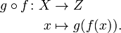
This notation follows the form such that .

The function on the right acts first and the function on the left acts second, reversing English reading order. We remember the order by reading the notation as "g of ƒ". The order is important, because rarely do we get the same result both ways. For example, suppose ƒ(x) = x² and g(x) = x+1. Then g(ƒ(x)) = x²+1, while ƒ(g(x)) = (x+1)², which is x²+2x+1, a different function.

In a similar way, the function given above by the formula y = 5x−20x³+16x⁵ can be obtained by composing several functions, namely the addition, negation, and multiplication of real numbers.

[edit] Identity function

Main article: Identity function

The unique function over a set X that maps each element to itself is called the identity function for X, and typically denoted by id_X. Each set has its own identity function, so the subscript cannot be omitted unless the set can be inferred from context. Under composition, an identity function is "neutral": if ƒ is any function from X to Y, then

[edit] Inverse function

Main article: Inverse function

If ƒ is a function from X to Y then an inverse function for ƒ, denoted by ƒ⁻¹, is a function in the opposite direction, from Y to X, with the property that a round trip (a composition) returns each element to itself. Not every function has an inverse; those that do are called invertible.

As a simple example, if ƒ converts a temperature in degrees Celsius to degrees Fahrenheit, the function converting degrees Fahrenheit to degrees Celsius would be a suitable ƒ⁻¹.

The notation for composition reminds us of multiplication; in fact, sometimes we denote it using juxtaposition, gƒ, without an intervening circle. Under this analogy, identity functions are like 1, and inverse functions are like reciprocals (hence the notation).

[edit] Specifying a function

A function can be defined by any mathematical condition relating each argument to the corresponding output value. If the domain is finite, a function ƒ may be defined by simply tabulating all the arguments x and their corresponding function values ƒ(x). More commonly, a function is defined by a formula, or (more generally) an algorithm — a recipe that tells how to compute the value of ƒ(x) given any x in the domain.

There are many other ways of defining functions. Examples include recursion, algebraic or analytic closure, limits, analytic continuation, infinite series, and as solutions to integral and differential equations. The lambda calculus provides a powerful and flexible syntax for defining and combining functions of several variables.

[edit] Computability

Main article: computable function

Functions that send integers to integers, or finite strings to finite strings, can sometimes be defined by an algorithm, which gives a precise description of a set of steps for computing the output of the function from its input. Functions definable by an algorithm are called computable functions. For example, the Euclidean algorithm gives a precise process to compute the greatest common divisor of two positive integers. Many of the functions studied in the context of number theory are computable.

Fundamental results of computability theory show that there are functions that can be precisely defined but are not computable. Moreover, in the sense of cardinality, almost all functions from the integers to integers are not computable. The number of computable functions from integers to integers is countable, because the number of possible algorithms is. The number of all functions from integers to integers is higher: the same as the cardinality of the real numbers. Thus most functions from integers to integers are not computable. Specific examples of uncomputable functions are known, including the busy beaver function and functions related to the halting problem and other undecidable problems.

[edit] Functions with multiple inputs and outputs

The concept of function can be extended to an object that takes a combination of two (or more) argument values to a single result. This intuitive concept is formalized by a function whose domain is the Cartesian product of two or more sets.

For example, consider the multiplication function that associates two integers to their product: ƒ(x, y) = x·y. This function can be defined formally as having domain Z×Z , the set of all integer pairs; codomain Z; and, for graph, the set of all pairs ((x,y), x·y). Note that the first component of any such pair is itself a pair (of integers), while the second component is a single integer.

The function value of the pair (x,y) is ƒ((x,y)). However, it is customary to drop one set of parentheses and consider ƒ(x,y) a function of two variables (or with two arguments), x and y.

The concept can still further be extended by considering a function that also produces output that is expressed as several variables. For example consider the function mirror(x, y) = (y, x) with domain R×R and codomain R×R as well. The pair (y, x) is a single value in the codomain seen as a cartesian product.

There is an alternative approach: one could instead interpret a function of two variables as sending each element of A to a function from B to C, this is known as currying. The equivalence of these approaches is expressed by the bijection between the function spaces and (C^B)^A.

[edit] Binary operations

The familiar binary operations of arithmetic, addition and multiplication, can be viewed as functions from R×R to R. This view is generalized in abstract algebra, where n-ary functions are used to model the operations of arbitrary algebraic structures. For example, an abstract group is defined as a set X and a function ƒ from X×X to X that satisfies certain properties.

Traditionally, addition and multiplication are written in the infix notation: x+y and x×y instead of +(x, y) and ×(x, y).

[edit] Function spaces

The set of all functions from a set X to a set Y is denoted by X → Y, by [X → Y], or by Y^X.

The latter notation is motivated by the fact that, when X and Y are finite, of size |X| and |Y| respectively, then the number of functions X → Y is |Y^X| = |Y|^|X|. This is an example of the convention from enumerative combinatorics that provides notations for sets based on their cardinalities. Other examples are the multiplication sign X×Y used for the cartesian product where |X×Y| = |X|·|Y| , and the factorial sign X! used for the set of permutations where |X!| = |X|! , and the binomial coefficient sign used for the set of n-element subsets where

We may interpret ƒ: X → Y to mean ƒ ∈ [X → Y]; that is, "ƒ is a function from X to Y".

[edit] Pointwise operations

If ƒ: X → R and g: X → R are functions with common domain X and common codomain a ring R, then one can define the sum function ƒ + g: X → R and the product function ƒ ⋅ g: X → R as follows:

for all x in X.

This turns the set of all such functions into a ring. The binary operations in that ring have as domain ordered pairs of functions, and as codomain functions. This is an example of climbing up in abstraction, to functions of more complex types.

By taking some other algebraic structure A in the place of R, we can turn the set of all functions from X to A into an algebraic structure of the same type in an analogous way.